Simulation
In this simulation you can visually learn about the phenomenon of gravitational lensing. We call gravitational lensing to the deflection of photons as they pass through the warped space-time of a gravitational field. Light rays from distant sources are not straight (in an Euclidean frame) if they pass near massive objects, such as stars, clusters of galaxies or dark matter, along our line-of-sight. We can see it if we look to the sky when there is a mass (lens) between us and another cosmological mass (source). The lens’ gravitational field curves the photons coming from the source and so we can see the source distorted, magnified and in a different position from where it really is.
In the simulation you can examine the effect caused by a lens in three different cases:
1. A point-mass lens and a point mass source
2. A point-mass lens and an extended source
3. A softened isothermal sphere lens and an extended source
Initially there appears the first case, but you can pass to the other two by opening the list and choosing the one you’d like to explore.
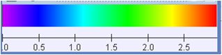
In the three cases the left graph is the source plane with the source and the caustics. On the right graph there is the lens plane with the image or images produced by the source on the left graph and the critical curves. It is supposed that the lens is located in the origin of the lens plane. Below the graphs there are some variables you can change by introducing a value different from the one imposed. You can see how it changes the lensing phenomenon. To observe what happens when the source approaches the lens (they can be very far away from each other but we consider what we would see when looking at the sky: lens, source and image in the same plane), you can change the values of the variables βx and βy or you can drag the source with the mouse where you want. You will see that the image changes as you change the position of the source. There is a selector button that makes critical curves and caustics appear or disappear, as these curves are only for guidance; they aren't part of the phenomenon. There is also another selector, which makes the magnification of the images appear or disappear. When it is clicked you can see the images with the different brightnesses in different bands; otherwise the whole image appears in the same color (yellow). The scale of the magnification:
Purple indicates the less magnification and red the most magnification zone. There is a reset button which doesn’t change the lens model, it only recovers the variables’ initial values. Up on the right there is a slider that acts as a zoom to change the scale of the graphs. The variables that appear on the presentation are:
• M → The lens’ mass
• Ds → The distance between the source and the observer
• Dd → The distance between the lens and the observer
• Dds → The distance between the lens and the source
• Radiusx → The extended source’s radius on the x direction
• Radiusy → The extended source’s radius on the y direction
• Centerx → The extended source’s center’s x coordinate
• Centery → The extended source’s center’s y coordinate
• σv → The velocity dispersion of the stars forming the softened isothermal sphere lens
• θc → The softened isothermal sphere’s core’s angle
• βx → The source’s x coordinate in the case of a point-mass source
• βy → The source’s y coordinate in the case of a point-mass source
θc is fixed by the values of Dds, Ds and σv. Ds is fixed by Dd and Dds. So they can’t be changed in the presentation; all the others can. If you put the mouse's cursor on a variable or on a graph, an explanation of it will appear.